Sometimes you can’t get everything you want. Here’s an afternoon hackathon project that challenged me to make the most of what I had.

We’ve all heard it before - you can get something fast and cheap, but it probably won’t be very good; you could get something good and cheap, but it will take a long time; or you can get something good and fast, but it’s going to cost you. In that vein, I participated in an afternoon hacking challenge that prompted us to predict whether a person’s salary was above $50,000.

But there was a catch: each of the three teams were handicapped by a constraint. ‘Team Samples’ was limited to the number of samples they were allowed to train on but could engineer an unlimited amount of features and choose their own models. ‘Team Features’ was bound to the number of features they could use (engineered or pre-existing) but could train on the full set of data and choose their own model. ‘Team Algorithm’ was not bound by the number of features or samples but was constrained by the model they were allowed to use. None of the three teams knew which team they were on until after the class had voted on the parameters of the constraint. While these constraints were not dealbreakers, they were highly unfavorable.

I was randomly assigned to ‘Team Features’ and constrained to using only three features from the dataset. In three and a half hours, I worked with my two teammates to build out the best model we could given our project and time constraints. Below is a summary of what we did that afternoon.

Ready? Go!

The dataset had 30,298 rows across 14 columns related to demographic information of workers, such as age, sex, education, marital-status, and occupation, to name a few. In a separate target set, we were given their corresponding salaries. Thankfully, there were no null values, which I would have likely dropped given the time constraint of the project.

There were eight categorical columns and six numerical columns. I decided to LabelEncode all of the categorical data in order to get the data into a model as quickly as possible.

With my data in numbers I could model with, I applied SelectKBest to the data and the salaries as my target. Given that I was constrained by the number of features I could feed into a model, I set my k value to three. SelectKBest identified that the three most predictive features of a salary were ‘education-num’, ‘relationship’, and ‘capital-gain’. To be honest, this surprised me, as I was expecting to see ‘sex’ as a major predictor. From there, I scaled and train-test-split my data before feeding it into a model. Given that this project was a competition, I wanted to challenge myself to use a new model that I hadn’t yet tried.

Power Up!

XGBoost, short for eXtreme Gradient Boosting, is a powerful algorithm used in many Kaggle competitions and is known for its performance as well as computational speed. The XGBoost algorithm is an ensemble model based on a Decision Tree methodology that creates new models based on predictions of errors from prior models and adds them together sequentially to make a final prediction. To calculate those errors, XGBoost employs the gradient descent algorithm which identifies optimal parameter values that minimize loss.

More specifically, gradient descent is an iterative method that chooses a random parameter value to optimize from a starting point dictated the user and calculates the loss of the function for that parameter value. It continues to randomly guess values for parameters until the loss is sufficiently minimized, meaning that the difference of loss function between two iterations of parameters is sufficiently small. The distance between one guess and the next is determined by the learning rate. Move too fast, however, and the algorithm might just skip over the best possible value, move too slowly, and the model might never converge. If the model fails to converge, the learning rate (alpha) will need to be increased.

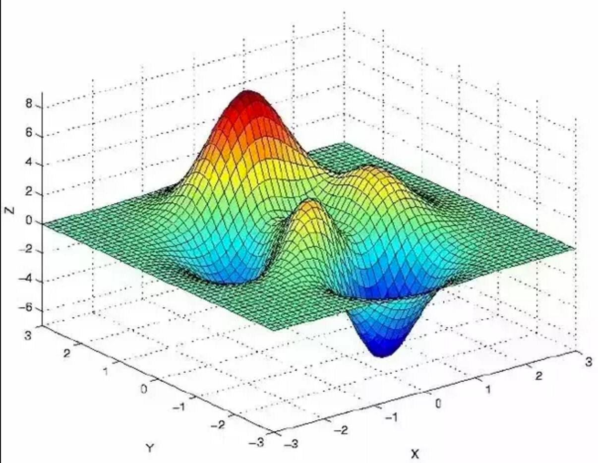
To understand this process visually, imagine yourself on a sled at the top of the peak in the graph below. Gradient descent will pick a random direction and sled down the mountain a little bit, calculate the loss function, and then sled down the mountain some more until it reaches a valley that satisfies the loss threshold, set as one of the parameters within the algorithm. XGBoost prevents the potential for overfitting by using L1 and L2 regularization penalties.¹

And the Winner Is…

When modeling my data using XGBoost, I also GridSearched across some parameters, namely ‘max_depth’, ‘n_estimators’, ‘learning_rate’ , and ‘booster’ to hypertune the model. The fitting took about four and a half minutes across 13,500 possible fits and returned the following best parameters:

• ‘booster’: ‘gbtree’,
• ‘learning_rate’: 0.7054802310718645,
• ‘max_depth’: 5,
• ‘n_estimators’: 10

The model scored a 0.847 for the training set and a 0.851 for the test set within the initial train-test-split.

Having fit the model and verified that it wasn’t overfit, we then applied our fitted XGBoost model to the hold-out test set and waited for our final score - a 0.841! Not bad for a model with only three features!

This was a really fun afternoon project and a great introduction to what Data Science might be like in a professional setting - I suspect that as a Data Scientist, I will have to make (and defend) all sorts of decisions when faced with client deadlines, budget constraints, and incomplete or limited datasets. Plus, it challenged me to learn a new and powerful model that I later applied to larger-scale projects.

To view the underlying code for this post, check out the corresponding GitHub repo.