When buying a new home, everyone wants the most bang for the buck. To that end, I analyzed homes in Ames, Iowa to identify what features of a house contribute the most to its sale price.

Buying a house is one of life’s most significant milestones, and according to the most recent census report on residential vacancies, around 64% of homes are occupant-owned.¹ But within the homeownership population, there is a wide range of what is considered desirable in a home which is unique to each home buyer. Some might want more bedrooms to accommodate a larger family. Others might want more garage space to fit their growing car collection. And still others might want a wrap-around porch for those hot summer nights. Regardless of individual preferences, however, it seems safe to assume that everyone wants the most bang for their buck. To that end, participated in a private Kaggle challenge during which I analyzed a dataset of homes located in Ames, Iowa to identify what features of a house contribute the most to its sale price.

Building the Foundation

To start, I wanted to get a sense of what the dataset looked like, both externally and internally. The initial shape of the data consisted of 2051 rows and 234 columns, with both numerical (numbers) and categorical (words) data. I knew I would need to convert the categorical data into a form that I could later feed into a model, but first, I wanted to see if I had any null values to contend with. Sure enough, both my numerical and categorical columns had null values, as seen in the plot below.

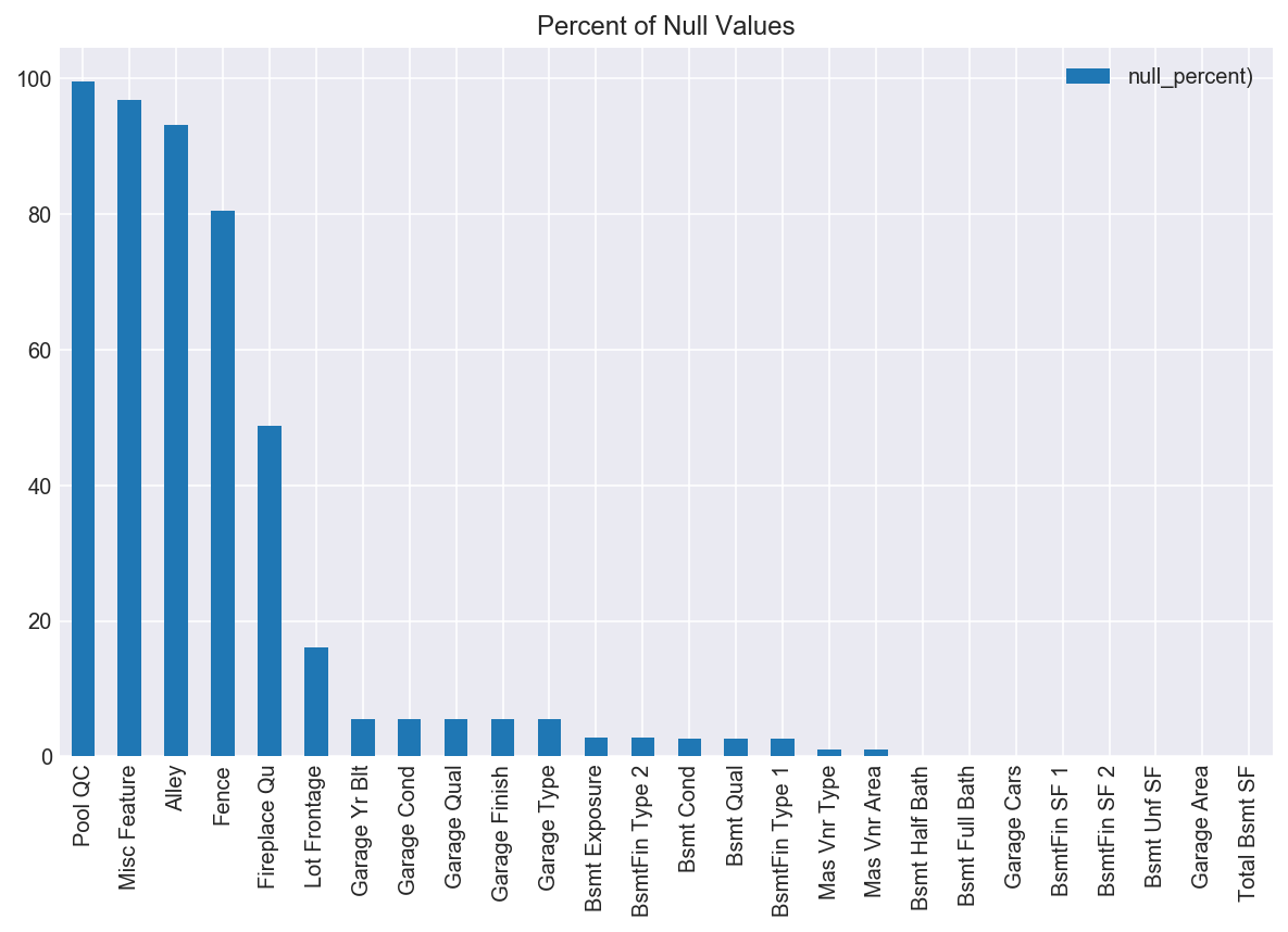
Based on the fact that ‘Pool QC’, ‘Misc Feature’, ‘Alley’, and ‘Fence’ all were missing over 80% of their data, I decided to drop those columns entirely, thinking that what few values existed in these columns would not be enough to inform the model one way or another, and would also not be statistically significant from which to impute new data.

For the rest of the columns, I decided to impute the missing data based on the data I had with the fancyimpute package which creates values that mimics the characteristics of values similar to them using a k-nearest neighbors distance calculation. This is similar to another technique related to upsampling the minority class that I’ve used in other projects.

I first imputed the numerical columns given that the data was already in the correct data type. I decided to use 3 k-nearest neighbors for calculation purposes and saved the imputed (and existing) data in a dataframe called ‘imputed_numerical’ which I decided to tack on to the initial train dataframe later.

The categorical columns, however, were not as easy to impute. Because fancy impute only takes in numbers, I decided to effectively “LabelEncode” my values while simultaneously skipping over the null values (so as not encode them and nullify the imputation exercise) using the following code snippet:

With my string values encoded with numerical values, I imputed the remaining null values with nine k-nearest neighbors. Having imputed all of the missing values, I then dropped the columns in the train set with the missing values and concatenated both the imputed_numerical and imputed_categorical onto the train dataframe, effectively replacing the initial columns with the missing values. I dummified the categorical columns that were not missing data to try to maintain as much interpretability as possible by assigning a new column to each unique value in the categorical columns. Having finished cleaning the data, it was ready to be fed into some models.

Choosing the Framework

Because I was most interested in which features contribute the most to a home’s price, I applied SelectKBest to the dataset. Unsurprisingly, the top ten features that are most predictive of a home’s sale price were: ‘Overall Qual’, ‘Year Built’, ‘1st Flr SF’, ‘Gr Liv Area’, ‘Garage Yr Blt’, ‘Total Bsmt SF’, ‘Garage Area’, ‘Garage Cars’, ‘Bsmt Qual’, and ‘Exter Qual_TA.’ Looking at these features, it makes sense that the overall quality of a home is most predictive of the value of a home, as does the square footage of the first floor, the basement, and garage area. Visually, we can see that these features are correlated to the sale price by plotting them on a heatmap.

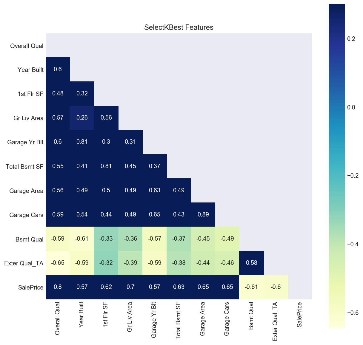
The bottom row on the left hand side of the plot follows the correlations of the SelectKBest features to the ‘SalePrice’ target. As we can see, Overall Quality is most positively correlated with Sale Price at a 0.8 correlation, followed by ‘Gr Liv Area’ with a score of 0.7, and so on. This means that when the values of these features increase, so too does the sale price of a home. Notably, ‘Bsmt Qual’ and ‘Exter Qual_TA’ were highly negatively correlated to ‘SalePrice’ meaning that when their values increase, the sale price decreases. The ‘BsmtQual’ feature measured the heights of basements, so based on this analysis, homebuyers don’t particularly value basements with high ceilings. The ‘Exter Qual_TA’ feature tracked homes with an exterior quality rated ‘TA’ - short for Typical/Average. Based on this finding, it appears that the sale price of a home decreases when its exterior quality is only rated ‘Average’ as opposed to ‘Excellent’ or ‘Good.’

No matter how complicated a data science project is, I always find it useful to take a step back sometimes and ask myself whether the results make sense. Machine learning isn’t some magical black box (although sometimes it feels that way) but rather, it’s a tool that extends the human analytical capabilities to crunch numbers faster and across far larger datasets than anyone has time for manually.

Having checked the top ten features, I then used SelectKBest to identify the top 100 most predictive features of a home’s sale price to feed into the model. I then polynomialized those features to capture the information gained from the interactions between features. I limited the features I polynomialized to 100 out of concern for computation issues.

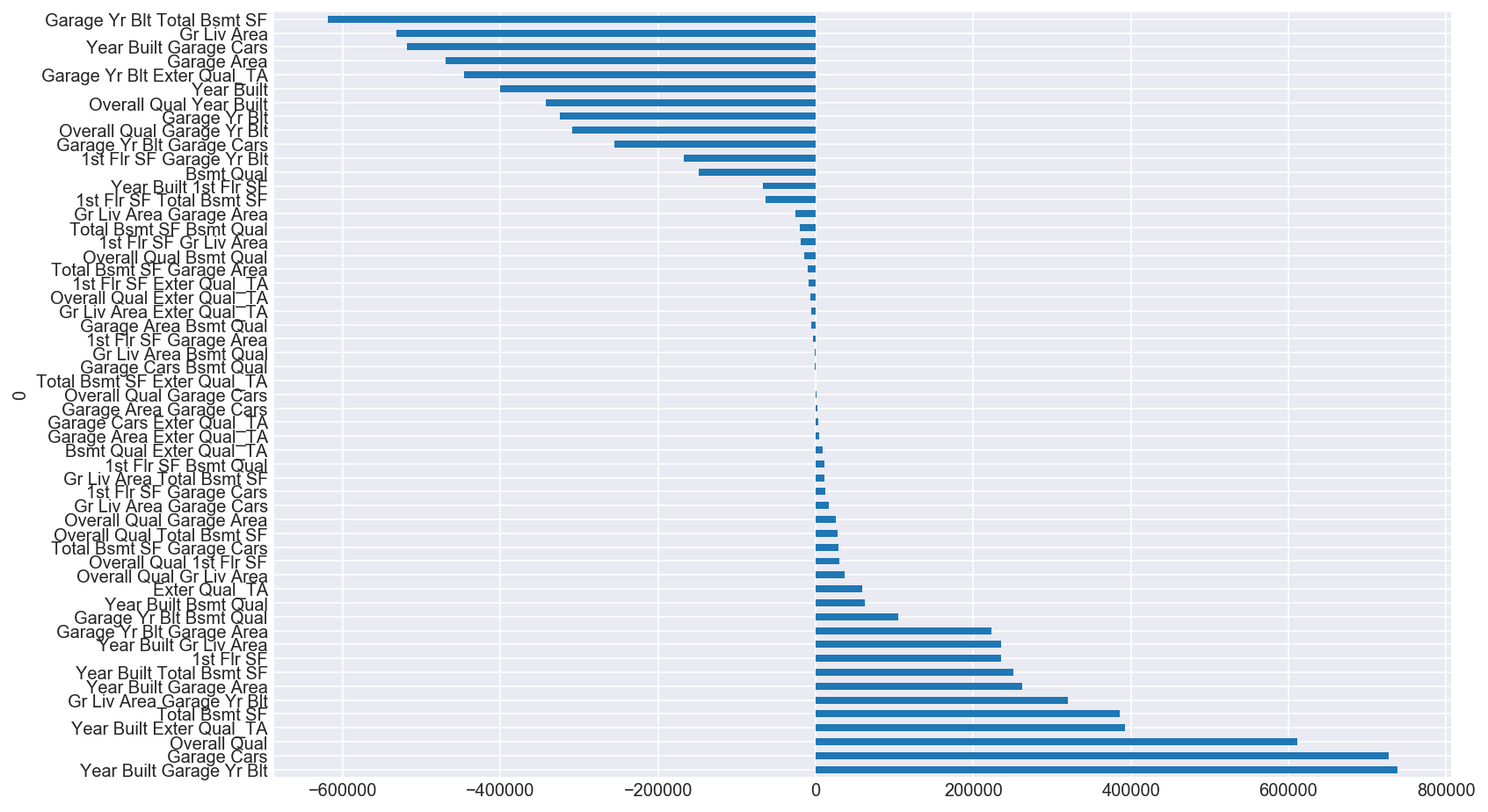
For illustrative purposes, I plotted the SelectKBest top ten features that I then polynomialized and zipped them to the coefficient values of the linear regression model without regularization. In the models that I actually ran, I included the top 100 polynomialized features but, because of computation (and space) issues, was not able to plot them in the same manner. As you can see, the coefficients varied widely and needed to be regularized.

Crunching the Numbers

Without regularizing my coefficients, my Linear Regression model scored a -3.154, which isn’t a viable R2 score and suggests that the model was overfit. To counter this issue, I used several different regularizing techniques, namely, Ridge, Lasso, and Elastic Net to “penalize” oversized coefficients in order to best minimize the loss function during model training. When loss functions are minimized, optimal coefficient values are revealed.

Another reason to regularize data is the fact that while features are correlated to the target to varying degrees, they can also be correlated to each other. Multicollinearity that goes unaddressed can affect the predictions made by the model and can be contingent upon small changes in sample sets that should not affect predictions. Moreover, variables that are correlated to each other cannot be independently interpreted as to how they contribute to the target, given that a change in one variable conditionally necessitates a change in another.

The Ridge regularization technique handles multicollinearity by penalizing the coefficients and effectively crunches them down. Lasso also addresses multicolinearity, but in a different way. Instead of “crunching” down the coefficients, it “zeroes” out the coefficients that are not statistically significant in predicting the target value. In effect, Lasso acts as a feature selector by zeroing out redundant or unimportant variables. The Lasso regularization technique was particularly useful in this dataset given that polynomializing the top 100 features identified by SelectKBest produced 5,050 features all together. Lasso pared this number down to 75 features, illustrated in the plot below.

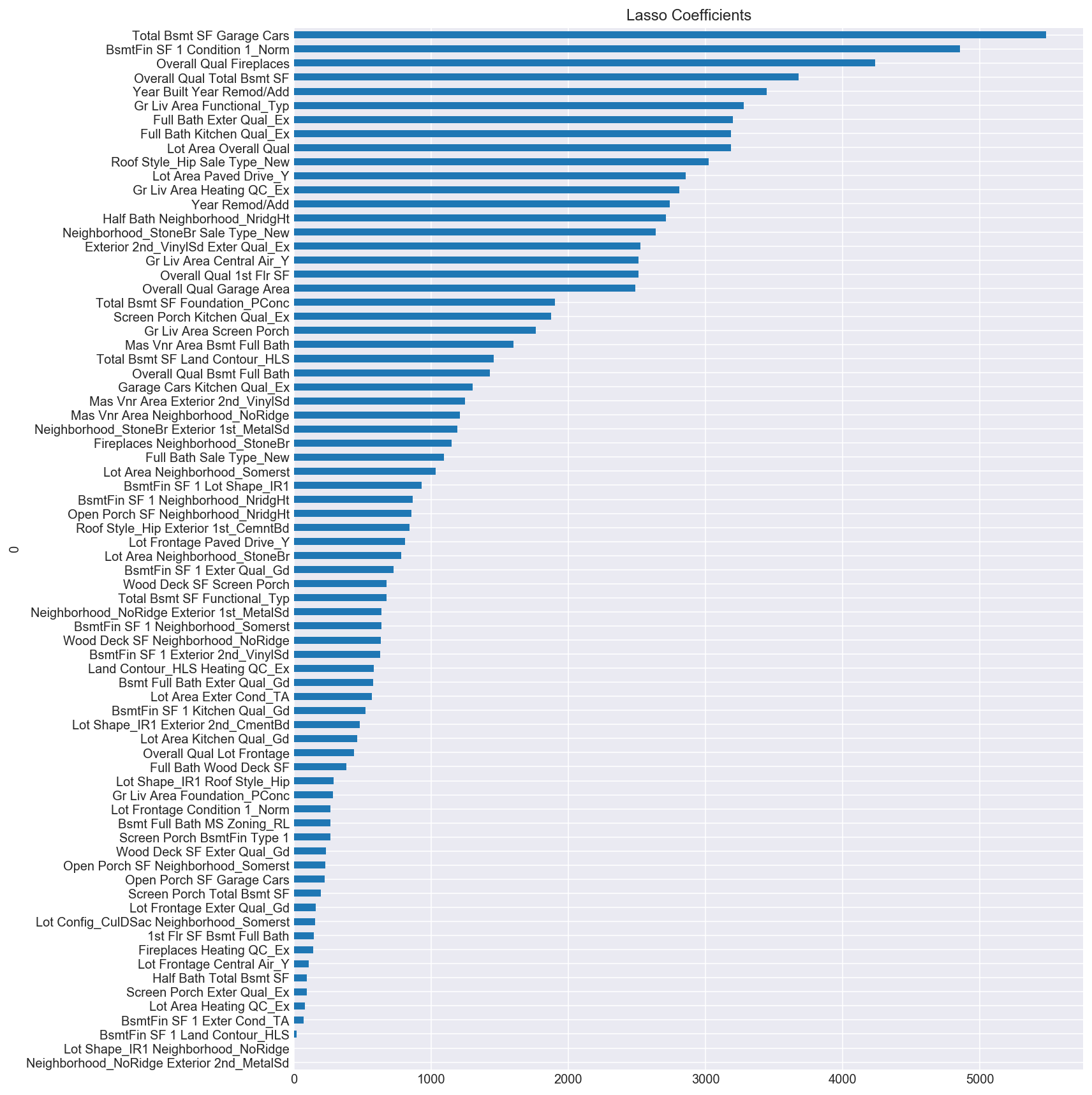
With the exception of dropping the Overall Qual Gr Liv Area polynomialized feature which had a coefficient value of 25000, the remaining 74 features ranged from just above 0 to 5000 (as opposed to -600,000 to over 700,000 in the first linear regression plot of the top ten polynomialized features.) This model is particularly useful when interpretability (as in the case of buying a house) is important.

I also ran an Elastic Net regression, which is a combination of both the Ridge and Lasso penalties.

Evaluating the Offer

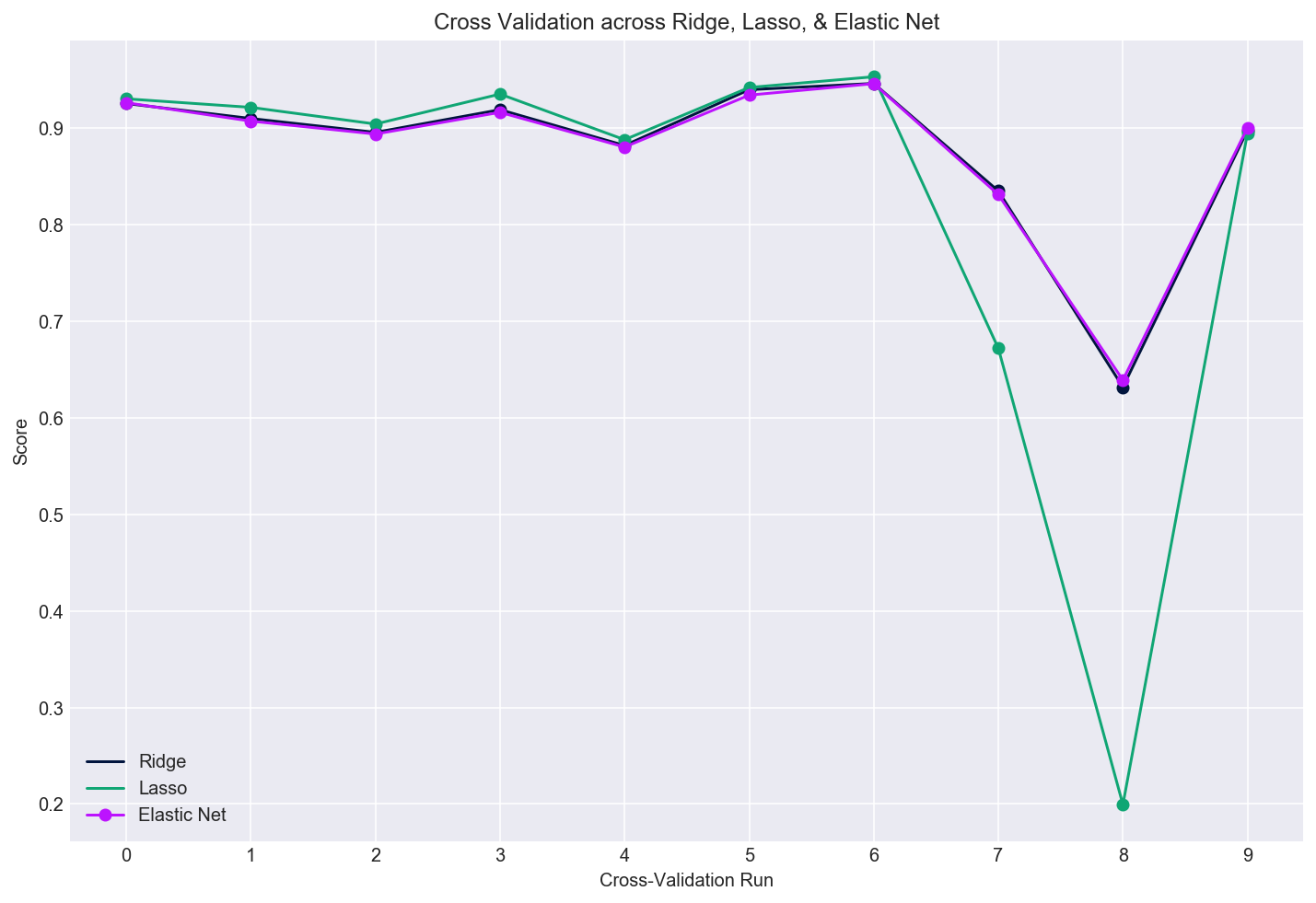
I ran 10 cross-validation runs across the three regularized regression models as seen in the plot below. It looks like all three models fared similarly, with the exception of Lasso’s ninth cross-validation run, where it fell down hard - perhaps because of the variation within the sample set it modeled.

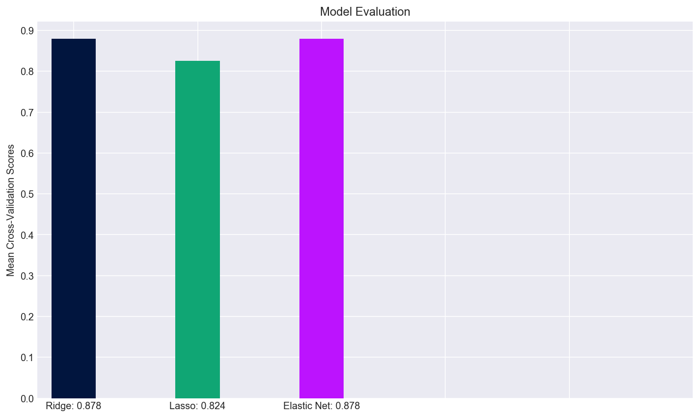
Put another way, I plotted the mean cross-validation scores of the three models in the bar plot below. Because of the ninth cross validation run of Lasso, it’s overall mean score was lower than that of the Ridge and Elastic Net models, however, it might still help a buyer choose a home given how interpretable the coefficients are.

Having conducted this analysis, it appears that the overall quality of a house, the amount of space in the living area, the square footage of the basement, whether there is a fireplace, and the year the home was built and/or remodeled all contribute greatly to the sale price of a house. In a future iteration of this project, I would be interested in analyzing which neighborhoods are considered most desirable based on their predictive values to the home’s sale price. Already, from the Lasso coefficients, we can see that the No Ridge and Stone Bridge neighbors have large coefficients, suggesting a statistical significance in their ability to predict a home’s sale price.

To view the code associated with this project, head on over to the corresponding GitHub repo