
Visions of the future are never completely true, but with the right key, some can be more truthful than others. Here’s an introduction to the neural network library, Keras, which I used to predict handwritten numbers.
When dreaming of the day her husband, Odysseus, would return from war, Penelope describes a vision she had that portends his return. Having waited twenty years already, she is wary of the dream’s validity, saying:
“Stranger, dreams verily are baffling and unclear of meaning, and in no wise do they find fulfilment in all things for men. For two are the gates of shadowy dreams, and one is fashioned of horn and one of ivory. Those dreams that pass through the gate of sawn ivory deceive men, bringing words that find no fulfilment. But those that come forth through the gate of polished horn bring true issues to pass, when any mortal sees them.” Homer, Odyssey 19. 560–569 ff (Murray translation)
Penelope describes dreams that pass through the ivory gates as deceitful whereas those that pass through gates of horn can be trusted. As Arthur Murray notes, the Greek word for horn, κέρας, recalls a similar sounding word κραίνω meaning “fulfill” whereas ἐλέφας, the Greek word for ivory, similarly recalls the word ἐλεφαίρομαι meaning “deceive.” Finally, my degree in Ancient Greek paid off.
François Chollet, a Google enigeer, drew inspiration from this imagery which was first referenced in the Odyssey nearly three thousand years ago when naming his popular neural network library, Keras. Designed explicitly for ease of use and speed, Keras is a deep neural network library that makes use of TensorFlow on the backend.
For my first neural network project, I applied Keras to the MNIST (“Modified National Institute of Standards and Technology”) handwriting database made available by Kaggle to predict numbers based on their handwritten equivalent. Below is a walkthrough of the steps I took to make predictions.
Prepping the Canvas
To start, I read the training set into pandas, identifying 42,000 rows and 785 columns of data, inclusive of the target column, ‘label.’ With the exception of the target column, all of the rest of the columns were pixel features of the images.
Because Keras requires a numpy array (as opposed to a pandas dataframe), I transformed the X set into a numpy matrix and then normalized the dataset by dividing each value by the maximum number of pixels (255). I also transformed the target (y) values into a one-hot encoded matrix given that this dataset is a multi-classification problem.
Before feeding the data into the neural network model, I train-test-split my data for training purposes.
Adding Nuance
I initialized the model by making it Sequential() and adding layers to it. Within a neural network, there are different layers that can be added to improve model performance. First, I added a dense layer which connected all of the neurons. Then, I added a “hidden” dropout layer. A hidden layer does not mean that it is not present or isn’t working - it just means that it is not the initial input layer or the final output layer, as seen in the image below.
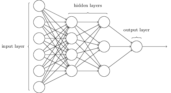
A neural network can have any number of hidden layers with any number of neurons. However, within each layer, each neuron will transform the data in different (and difficult to quantify) ways based on the assigned and change in weights within that neuron.
I decided to set my dropout layer to 0.5, which means that 50% of the neurons would be randomly “turned off” from training. I did this to prevent the model from being overfit to the training set and to allow for some flexibility when faced with new data.
model = Sequential()
model.add(Dense(X_train.shape[1], input_shape=(784,), activation='relu'))
model.add(Dropout(.5))
model.add(Dense(y_train.shape[1], activation='softmax'))
Next, I activated the training set with ‘relu’ (Rectified Linear Unit) which only activates neurons whose output will be positive. For the target, I activated with ‘softmax’ to essentially normalize the inputs within a scale of 0 to 1 to create a probability for an input falling within one of the target classes.
Knowing Your Audience
The next step to modeling a neural network is to compile the model. I chose the ‘adam’ optimizer given its ease of use, computational efficiency, and ability to handle large sets of data. While there is much more complex math behind how ‘adam’ is derived, essentially it works similar to (but different from) stochastic gradient descent in which the loss function is computed during each epoch and, as a result, neurons are re-weighted until the loss is sufficiently minimized. ‘Adam’ differs slightly from stochastic gradient descent by incorporating a dynamic and adaptive learning rate determined by the magnitude of change to the gradients.1
Because this was a muticlassification problem, I set the loss metric to ‘categorical_crossentropy’ as suggested by the Keras documentation.
Failing Better
When training the model, a user can specify how many epochs used to train the model. An epoch is a “roundtrip” for information to be passed forwards and backwards through the network.
During forward propagation, data is passed from the initial input layer, through the hidden layers, and finally to the output layer during which weights, biases, and activation functions are applied to the neurons.
During back propagation, the data is then passed back from the output towards the input layer, measuring the loss produced from the weights assigned to the neurons and, using gradient descent, changes the weights accordingly in order to make more accurate predictions over a user-defined number of iterations. The amount of epochs to use during training can be identified when either the accuracy or the loss of the predictions stabilizes at an acceptable value.
To illustrate this point, I plotted a summary chart of the four runs I conducted, tweaking the number of epochs and the dropout percentage with each new run.
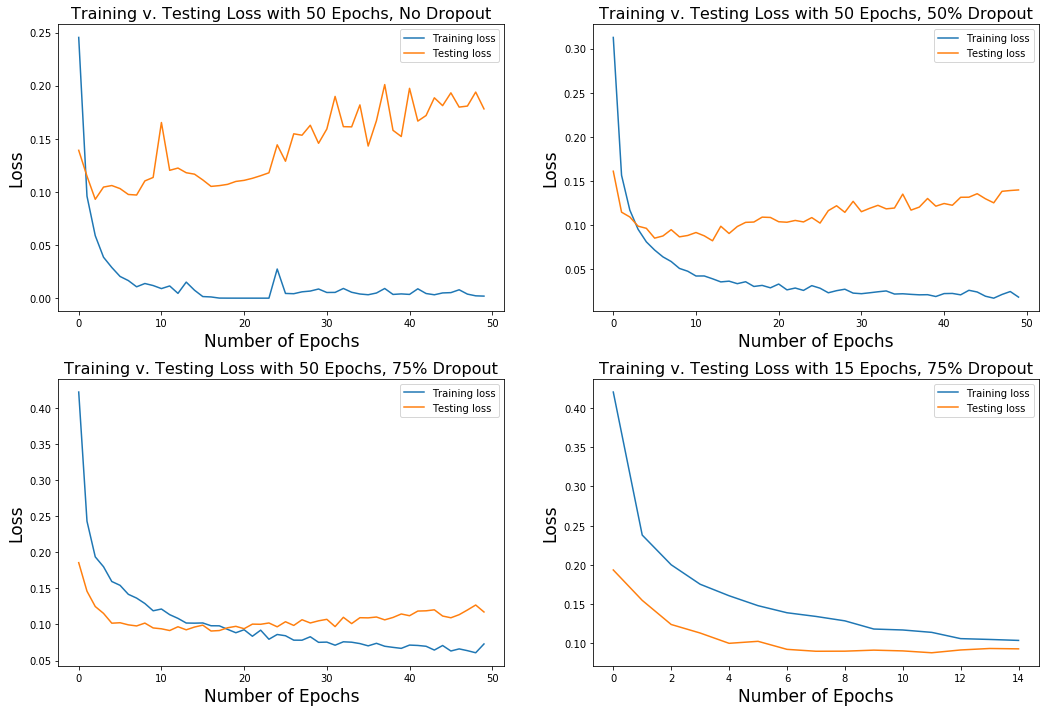
The top left plot shows the loss from both the training and the cross-validation (test) during which I trained 50 epochs without a dropout layer. Notice how the training loss dramatically reduces within the first ten epochs but continues to improve only slightly as the training continues to the 50th epoch. The loss from the test set, however, increases with the number of epochs with a wider amount of variance - a clear sign of overfitting. The top right plot shows a similar training run but with an added dropout layer of 50%. Both the training and test sets appear to be more stable and the loss from the test set is reduced. In my third run, illustrated by the bottom left plot, I increased the dropout percentage to 75% while still running 50 epochs. Again, the test loss amount is reduced. Finally, in the fourth run, noticing that in the last three runs there was a shift in performance between the tenth and twentieth epoch, I decided to set my training epochs to 15 while keeping the dropout rate at 75%. In this run, the test set loss hued closely to the loss of the training set. Now I had a model that was trained up on the dataset while remaining flexible enough to predict on unseen data. To further illustrate this point, I input the training and test loss values into a table for easier comparison.
| Run | Epochs | Dropout | Train Loss | Test Loss |
|---|---|---|---|---|
| 1 | 50 | 0% | 0.002 | 0.178 |
| 2 | 50 | 50% | 0.019 | 0.140 |
| 3 | 50 | 75% | 0.073 | 0.117 |
| 4 | 15 | 75% | 0.104 | 0.093 |
Art is a Lie that makes us Realize Truth
As machine learning continues to be integrated into our daily lives, we should be as discerning as Penelope was when determining which visions of the future are true and which are false.
To see all of the code associated with this post, check out the associated GitHub repo.