
SEC Filings
July 2018 »
The FBI and the American Association of Certified Fraud Examiners estimate that white collar crime costs 300 to 600 billion dollars a year. That’s the equivalent of Warren Buffet’s net worth 3.5 times over, or buying out the debt of New York City’s MTA 9 times over, or purchasing the New York Knicks 90 times over. It’s incredible amount of money and also a very wide range, suggesting that enforcement agencies don’t actually know the extent of the damage cause by white collar crime.
And that damage is not just limited to the crime itself - the ripple effects of financial crime are even wider, more opaque, and undoubtedly affects all of us. Companies that are defrauded will raise prices on consumer goods to recoup losses. Scammed insurance companies will demand higher premiums on their policies. Hedge fund schemes that manipulate equity markets can decrease stock prices. And if the government gets taken for a ride, well, we all know what happens then - more government taxes.
Identifying these bad actors is difficult. Complex financial schemes usually involve a lot of documents, some of which demand law or accounting degrees to truly understand. Moreover, as with many government agencies, there’s just not enough people to review all of those complex documents. And the select few who are tasked with reviewing these complex cases are doing it with outdated and insufficient technology.
Corporations that are listed on any U.S. stock exchange are required to submit financial reports to the Securities and Exchange Commission (SEC) to inform potential investors of the company’s financial health. There are hundreds of filing types that a corporation can submit, and these filings include information like quarterly and annual financial statements, major events, changes to the institution’s organizational structure, and foreign investments, to name a few. The SEC makes these filings publicly available on their website.
To that end, I wanted to use data science techniques like web scraping, exploratory data analysis, and machine learning to see whether I could identify ‘bad actor’ corporations by the types of reports they file in concert with other demographic information to help financial regulators like the SEC focus their investigations of white collar crime.
Identifying the Target
My first task was to identify my targets so I could train my model on what suspicious cases might look like. I researched SEC indictments reports and found that the SEC releases annual reports of their enforcement cases. For example, in these reports I found, there is a list of indictments with information about the defendant (either an individual or a corporation) as well as date information and related charges. I located reports for the years 2006-2016. Given that these reports were in pdf format, my first task was to find a way to extract the information I needed into a format that I could eventually feed into my model. I first tried using a package I found that reads in material from pdfs, but because of the inherent unstable process of extracting text, the formula I wrote to extract the text from the first report did not extract text in the same way as the next. Because I only had a couple of weeks to complete this project and needed to extract text from eleven reports just to identify my targets, I quickly abandoned this method. I later found a free website that more accurately (and quickly) converted my reports to excel files. In data science as in many disciplines, sometimes the simplest tool is the best.
The next big hurdle to overcome was the fact that names of individuals and corporations are not easily fed into searches. In a future iteration of this project, I would try to use some of kind fuzzing matching algorithm like the fuzzy wuzzy package to feed the names of the defendants into a search box.
For now, I manually entered the names of the cases into the EDGAR search field to identify their corresponding CIK ID Number. Because I didn’t want to manually search 5,000 entries, I pared my initial list of defendants down to corporations. Many of the names of the corporate defendants did not turn up a CIK number. (For some cases, this makes sense given that these corporations were accused of financial crime and may never have filed the required reports). From the 1600 or so corporate cases I had, I was able to identify 175 corporates with CIK ID numbers. I finally had my target set.
Putting the Case Together
But what about my Not Indicted class? If I was going to make predictions, I needed to build out my dataset with values associated with corporations that have not had enforcement action against them, given that that is the overwhelming norm. Initially, I thought about doing the same process over again with just a random list of companies from the S&P500, but after more research, I found a similar project that had already done some of the work that I wanted to. Given my time constraints, I decided to download their datasets, which also identifies corporations by the Central Index Key (CIK). These datasets contained the types of data points I was looking for, namely, locations and years active. I suspected that the 175 target corporations I had previously identified were somewhere in the 65,000 rows of corporates, so I subset my target data set out of the much larger dataset. When I compared the shapes of the prior set to the new set, sure enough, 175 rows were dropped. I created a new column within my new dataset called ‘Indicted’ and set it to ‘0’. Then, I concatenated my target dataset on the 0 axis with its corresponding ‘Indicted’ column and set it to 1, meaning, positive for having been indicted.
With the CIK ID numbers for both of my Indicted and Not Indicted classes, I was able to scrape the SEC website for their filings using a nested for loop with the requests and Beautiful soup libraries. Having saved all of my filings in a list for each of my 65,000 rows, I then transformed those individual filings into their own unique dummy columns and filled each column with the value counts of the filing. With this final transformation, I had a working dataset that I could analyze and subsequently feed into a model.
Witness Selection
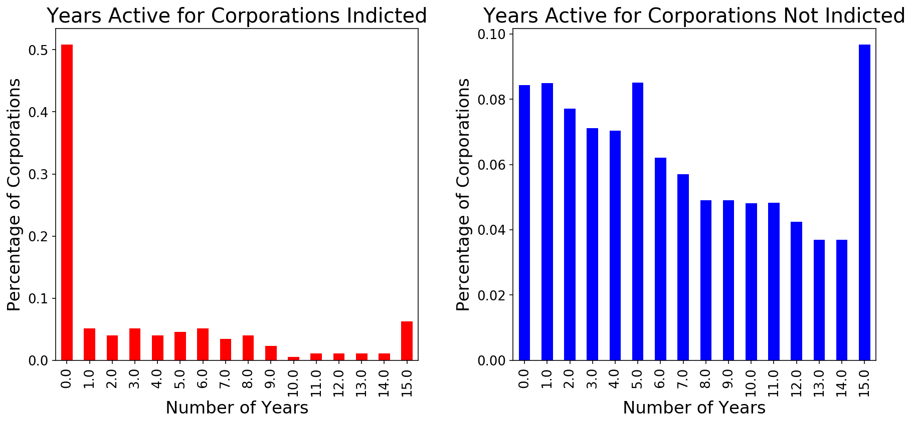
I knew that I was likely going to use some ‘blackbox’ models that would limit my ability to interpret what weights were given to which features in predicting the Indicted class. So, I decided to use a tool that does allow for interpretability of what factors are most predictive of the minority class. SelectKBest, identified features that were most predictive of my Indicted class. One of the top ten features identified was the number of years a corporation was active. As visualized in the plot below, half of the Indicted class was active for less than a year, whereas there is more of a normal distribution among the Not Indicted class.
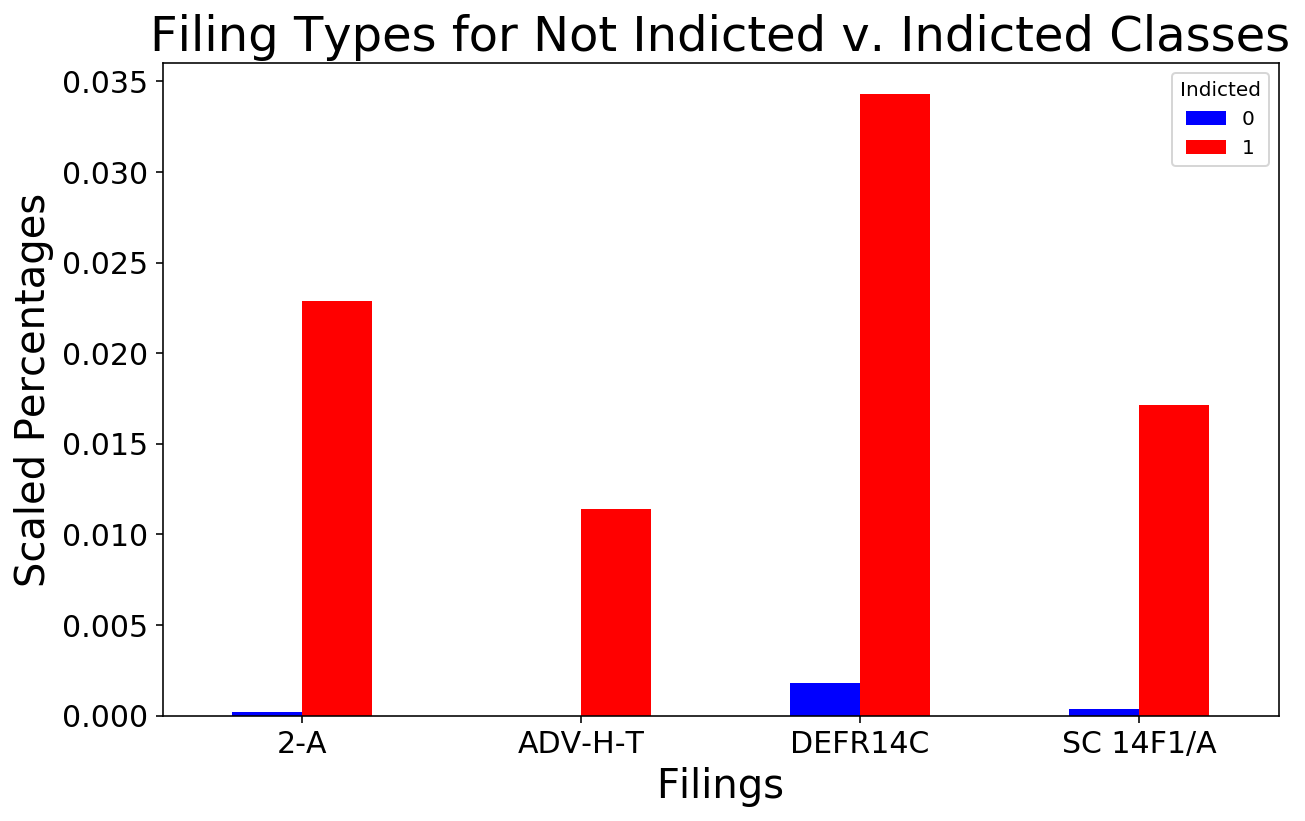
In addition to the number of years a corporation has been active, SelectKBest also identified several filing types that were highly predictive of the minority class, including the ‘2-A’, a report of sales and uses of proceeds,1, the ‘ADV-H-T’, an application for temporary hardship,2 the ‘DEFR14C’, a filing that discloses pertinent information that is required to be disclosed to shareholders but does not required a shareholder vote for approval,3 and the ‘SC 14F1/A’, a filing disclosing a majority change in a corporation’s directors.4
The Indicted class filed these types of filings with slightly more frequently than did the Not Indicted class, as illustrated in the plot below.
In analyzing the purpose of these filings, I posited that some corporations might be “hiding” pertinent information that in fact should be voted on by shareholders, or, in the case of the ‘SC 14F1/A’ registering the corporation with a ‘straw owner’ to give an air of legitimacy before the “real” directors take over to pursue potentially criminal activities.
Balancing the Scales
My baseline accuracy for this project was 99.7%. This means that if you guessed that a corporation was not indicted (0 in the target column), you would be right 99.7% of the time. With my majority and minority classes so imbalanced, it is difficult for the machine to pick up on the (very subtle) signals that the minority class is sending out. To counter-act this imbalance, I used several different class balancing techniques to amplify the minority class’s signals.
First, I used a resampling technique called downsampling from scikit-learn’s utils package. This technique allowed me to reduce the majority population to try to “quiet” the amount of signals the majority class sends out. I chose to downsample my majority class from 65,324 down to 10,000 and assumed that 10,000 samples of the majority class would have enough variety to represent the full 65,324 set.
With my majority class muffled a little bit, I then used another sampling tool called SMOTEENN to try to amplify the signals of my minority class (the Indicted class). Imblearn’s SMOTEENN is a slight variation of SMOTE (Synthetic Minority Oversampling TEchnique which randomly selects data points in the minority class and creates copies of them that mimic the characteristics of the minority class based on a k nearest neighbors distance calculation. SMOTEENN differs slightly from SMOTE by additionally using Edited Nearest Neighbors (ENN), which in essence “cleans” the data set of points that are not strong representatives of their class. Put another way, it reduces noise within the data set for both classes. I verified that the were properly balanced by checking their shapes. In fact, both had 10,892 rows of data.
I then performed two train-test-splits on the dataset - the first set would be used to initially train my models on my X_train and y_train. Within this first set, I would conduct another train-test-split on my X_train and y_train which would be split into my cross-validation set (X_train_val, y_train_val, X_test_val, y_test_val). Cross validating my models on a dataset that the model hasn’t been trained on guards against overfitting my models to any one particular dataset. If and when I was satisfied with the results of my models and satisfied with how my parameters were tuned, I would then predict on the X_test from the initial train-test-split - another dataset that the models have not yet seen.
Reaching a Verdict
When running my models, I decided to score on precision because I was most concerned with reducing false positives while also trying to increase the number of true positives as much as possible. The equation for precision, seen below, calculates the positive predictive value but penalizes the score by how many positive values were predicted incorrectly. In my project, a false positive would be a corporate that was predicted to be indicted but should not have been.
In a slightly different metric, recall measures the true positive rate by penalizing the score with false negatives (seen below). In this project, a false negative would be a corporate that should have been indicted but wasn’t.
In sum, both precision and recall are measures of truthiness but with slightly different perspectives. Because it is a much more serious thing to indict a corporation that is innocent (both in terms of potential monetary penalties when the corporation turns around and sues the government as well as lost faith in the justice system) than to not indict a potentially guilty corporation, I decided that precision was the most important measure of success.
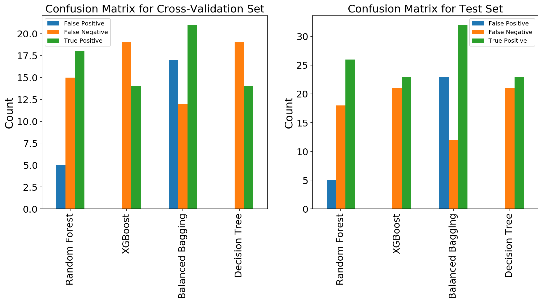
To visualize this decision, I plotted two confusion matrices of the models I ran to represent the cross-validation run (left) and the test run (right). Despite the name, a confusion matrix is actually quite a simple tool to interpret. Simply, it is a matrix of four values: true positives (values that were predicted positive and supposed to be positive), false positives (values that were predicted positive but supposed to be negative), true negatives (values that were predicted negative and supposed to be negative), and false negatives (values that were predicted negative but supposed to be positive) to compare the number of false positives, true positives, and false negatives. In the cross-validation run, both the Decision Tree and XGBoost Classifiers kept the false positives to 0 while predicting 14 true positives. They both left 19 false negatives on the table (corporations that should have been indicted but weren’t). The Random Forest and Balanced Bagging Classifiers both predicted more true positives (18 and 21, respectively) but they also predicted more false positives (5 and 17, respectively). In my mind, the benefit of indicting 4 to 7 more corporations does not outweigh the cost of inappropriately accusing 5 to 17 corporations (and the attendant damage caused to the company for being embroiled in litigation).
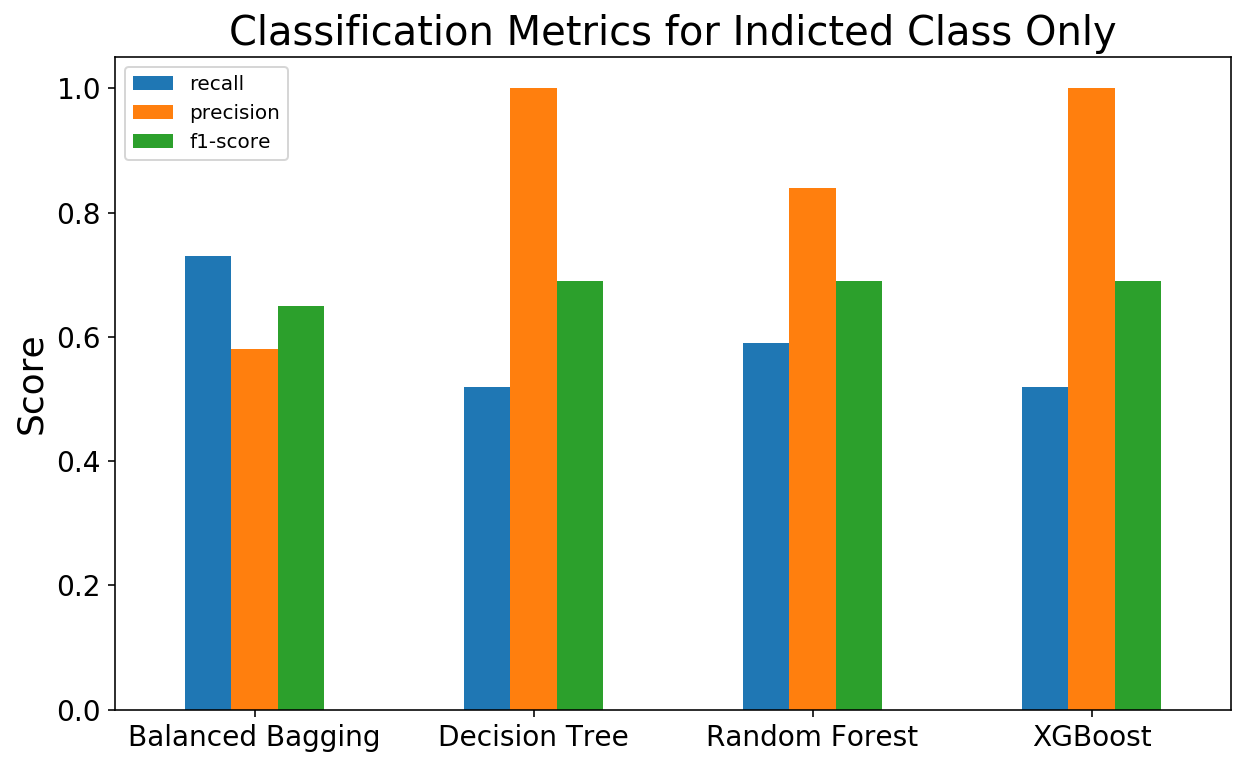
To focus in on the Indicted class even more, I also plotted the classification reports of each the models. Similar to a confusion matrix, a classification report is another tool that can be used to evaluate model performance other than accuracy. Some of the outputs of a classification report are: precision, recall, and an f1-score (a weighted average of the precision and recall metrics). Because the Decision Tree and XGBoost Classifiers both reduced false positives to 0, they have perfect precision scores of 1.0. However, because they both left corporations “on the table”, their recall scores are not as great. Because the goal of this project was to identify as many corporations as possible to further investigate without investigating a corporation that should not be, I considered these metrics a success.
Areas of Further Research
While this was a toy project based on a handful of inputs related to corporate demographics and filing types, I think it demonstrates the point that machine learning techniques can help financial regulatory agencies identify potential targets for further investigation. If I were to continue researching this topic, I would be interested in pulling in more data to feed the model, such as the names of the directors as well as any associated negative news. I would also be interested in “reading” the filings themselves using natural language processing, and specifically, a Term Frequency - Inverse Document Frequency (TF-IDF) analysis to identify any rare terminology that might signal unusual behavior.
To see all of the code associated with this project, head on over to the related GitHub repo.